Leonard Lobel (Microsoft MVP, Data Platform) is the chief technology officer and co-founder of Sleek Technologies, Inc., a New York-based development shop with an early adopter philosophy toward new technologies. He is also a principal consultant at Tallan, Inc., a Microsoft National Systems Integrator and Gold Competency Partner.
Programming since 1979, Lenni specializes in Microsoft-based solutions, with experience that spans a variety of business domains, including publishing, financial, wholesale/retail, health care, and e-commerce. Lenni has served as chief architect and lead developer for various organizations, ranging from small shops to high-profile clients. He is also a consultant, trainer, and frequent speaker at local usergroup meetings, VSLive, SQL PASS, and other industry conferences.
Lenni has also authored several MS Press books and Pluralsight courses on SQL Server programming
Before diving into the hands-on labs, ensure you have the necessary software and databases installed. Follow these steps to set up your environment:
SQL Server 2022: A local instance of SQL Server 2022 is required for the labs. The Developer Edition of SQL Server 2022 is free for development and testing, not for production, and includes all the features of SQL Server 2022. Download and install it from Microsoft’s SQL Server Downloads page. When the installer starts, choose the Basic installation option.
SQL Server Management Studio (SSMS): To interact with SQL Server, including running queries and managing databases, install the latest version of SSMS. This ensures compatibility with SQL Server 2022 and supports features like Always Encrypted that may not be supported in older SSMS versions. Download SSMS from here.
Visual Studio 2022 (any edition) with .NET desktop development workload: Some demos, especially those involving Row-Level Security and Always Encrypted, require Visual Studio 2022. The Community Edition is free for students, open-source contributors, and individuals. Download it from Visual Studio’s Community Edition page. During installation, choose the “.NET desktop development workload.”
AdventureWorks2019 Database: Many demos utilize the AdventureWorks2019 sample database. Download the AdventureWorks2019.bak backup file available here. Then restore the backup file as follows:
Create a temporary folder First, create a temporary folder on your C drive to store the .bak file during the restoration process. In File Explorer, navigate to the C drive (C:). Then right-click in an empty space, select New > Folder, and name the new folder HolDB.
Copy the backup file Navigate to your Downloads folder. Right-click on the AdventureWorks2019.bak file and select Copy. Then go back to the C:\HolDB folder, right-click in an empty space, and select Paste.
Restore the Database using SSMS Now that the backup file is in an accessible location, you can proceed with restoring it to your SQL Server instance.
Open SQL Server Management Studio (SSMS) and connect to your local SQL Server instance.
In the Object Explorer on the left, expand and then right-click on the Databases folder and select Restore Database…
In the Restore Database Dialog, select the Device radio button under the Source section.
Click the ... button on the right to open the Select Backup Devices dialog.
Click on the Add button to open the Locate Backup File dialog.
Navigate to the C:\HolDB folder and select the AdventureWorks2019.bak file, then click OK.
The backup file should now appear in the Select Backup Devices dialog. Click OK to return to the Restore Database dialog.
Now click OK to start the restore process.
The restoration process will begin, and SSMS will display a progress bar. Once the process completes, a message will appear informing you that the database has been successfully restored. Click OK, and the AdventureWorks2019 database will appear in the Databases folder in Object Explorer.
Wide World Importers Database: One lab uses the Wide World Importers sample database. Download the WideWorldImporters.bak backup file file available here. Then restore the database using similar steps you just followed for AdventureWorks2019:
Copy the Backup File Copy the WideWorldImports.bak file from your Downloads folder to the C:\HolDB folder.
Restore the Database using SSMS
In the SSMS Object Explorer, right-click on the Databases folder and select Restore Database…
In the Restore Database Dialog, select the Device radio button under the Source section.
Click the ... button on the right to open the Select Backup Devices dialog.
Click on the Add button to open the Locate Backup File dialog.
Navigate to the C:\HolDB folder and select the WideWorldImports.bak file, then click OK to return to the Select Backup Devices dialog.
Click OK to return to the Restore Database dialog.Click OK to start the restore process.
After the restore completes successfully, the WideWorldImporters database will appear in the Databases folder in Object Explorer.You can now delete the C:\HolDB folder, as well as the two database backup files in your Downloads folder.
Dynamic Data Masking (DDM) is a security feature introduced back in SQL Server 2016 that obscures sensitive data in the result set of a query, ensuring that unauthorized users can’t see the data they shouldn’t access. See my older blog post at https://lennilobel.wordpress.com/2016/05/07/sql-server-2016-dynamic-data-masking-ddm/ for an introduction to this feature. This blog post explains the new DDM capabilities added in SQL Server 2022; specifically, granular permissions.
For example, here is a table with four masked columns, populated with a few rows of data:
-- Create table with a few masked columns CREATE TABLE Membership( MemberId int IDENTITY PRIMARY KEY, FirstName varchar(100) MASKED WITH (FUNCTION = 'partial(2, "...", 2)') NULL, LastName varchar(100) NOT NULL, Phone varchar(12) MASKED WITH (FUNCTION = 'default()') NULL, Email varchar(100) MASKED WITH (FUNCTION = 'email()') NULL, DiscountCode smallint MASKED WITH (FUNCTION = 'random(1, 100)') NULL)
In order for a user to see the data in the four masked columns, they must be granted the UNMASK permission. However, prior to SQL Server 2022, this was a database-wide permission; users that have the UNMASK permission can see every masked column in every table of every schema in the database.
The granular DDM permissions feature introduced in SQL Server 2022 is a significant enhancement that addresses this major limitation. Previously, SQL Server allowed granting or revoking the UNMASK permission only at the database level, which limited its flexibility and adoption. However, SQL Server 2022 expands this capability, offering much-needed granularity. Now, administrators can grant or revoke UNMASK permissions at various levels, providing tailored access control that matches specific security requirements.
This granular control can be applied:
Database Level: As before, affecting all masked columns across the entire database.
Schema Level: Affecting all tables within a specific schema.
Table Level: Applying to all columns within a specific table.
Column Level: The most granular level, targeting individual columns within a table.
This flexibility greatly enhances the practical use of Dynamic Data Masking by allowing precise control over who can see unmasked data, ensuring that only authorized users can access sensitive information at the level of detail appropriate to their role or needs. Let’s see how to grant UNMASK permissions at the individual column level.
We’ll set column-level UNMASK permissions for a specific user, named ContactUser, who has been tasked with reaching out to members. To facilitate this, they’ll need access to certain information that’s normally masked, specifically the FirstName, Phone, and Email columns within the Membership table. However, they don’t require access to the DiscountCode, which should remain masked:
-- Create a new user called ContactUser with no login
CREATE USER ContactUser WITHOUT LOGIN

-- Grant SELECT permissions on the Membership table to ContactUser
GRANT SELECT ON Membership TO ContactUser

-- Grant UNMASK permission on specific columns to ContactUser
GRANT UNMASK ON Membership(FirstName) TO ContactUser
GRANT UNMASK ON Membership(Phone) TO ContactUser
GRANT UNMASK ON Membership(Email) TO ContactUser
By running the above code, we’ve created ContactUser and granted them the SELECT permission on the Membership table. We’ve then gone a step further by granting the UNMASK permission, but specifically and only for the FirstName, Phone, and Email columns. This allows ContactUser to view these normally masked columns in their unmasked state, while the DiscountCode remains masked, adhering to the principle of least privilege.
Let’s see what happens when ContactUser accesses the Membership table, particularly focusing on the columns for which they’ve been granted UNMASK permissions:
-- Impersonate ContactUser to query the Membership table
EXECUTE AS USER = 'ContactUser'
SELECT * FROM Membership
REVERT
By executing the code above, you’ll notice that ContactUser can view the FirstName, Phone, and Email columns without any masking, thanks to the granular UNMASK permissions that have been explicitly granted for these columns. However, the DiscountCode remains masked, with its values randomized between 1 and 100, demonstrating the effect of the random() masking function. This behavior aligns perfectly with our intent for ContactUser, allowing them access to the necessary contact information while keeping other sensitive data, like discount codes, masked. Run the code multiple times to observe the dynamic masking in action for the DiscountCode column.
Granular DDM permissions can also be granted at the schema and table level. For example:
-- View unmasked data in all columns of all tables in the dbo schema
GRANT UNMASK ON SCHEMA::dbo TO SomeUser

-- View unmasked data in all columns of the Membership table in the dbo schema
GRANT UNMASK ON dbo.Membership TO SomeUser
This new ability in SQL Server 2022 significantly enhances the usefulness of Dynamic Data Masking in SQL Server 2022. Happy coding!
Partitioning is a critical core concept in Azure Cosmos DB. Getting it right means your database can achieve unlimited scale, both in terms of storage and throughput.
You need to define a partition key for your container, which is a property the every document contains. The property is used to group documents with the same value together in the same logical partition.
NoSQL databases like Cosmos DB do not support JOINs, which requires us to fetch related documents individually, and that becomes problematic from a performance standpoint if those documents are scattered across a huge container with many partitions, requiring a “cross-partition” query. But if the related documents all share the same partition key value, then they are essentially “joined” in the sense that they are all stored in the same logical partition, and therefore they can be retrieved very efficiently using a “single-partition” query, no matter how large the container may be.
Containers are elastic, and can scale indefinitely. There is no upper limit to the number of logical partitions in a container. There is, however, an upper limit to the size of each logical partition, and that limit is 20 GB. This limit is usually very generous, as the general recommendation is to choose a partition key that yields relatively small logical partitions which can then be distributed uniformly across the physical partitions that Cosmos DB manages internally. However, some scenarios have less uniformity in logical partition size than others, and this is where the new hierarchical partition key feature just announced for Azure Cosmos DB comes to the rescue.
Before Hierarchical Partition Keys
Let’s use a multi-tenant scenario to explain and understand hierarchical partition keys. Each tenant has user documents, and since each tenant will always query for user documents belonging just to that tenant, the tenant ID is the ideal property to choose as the container’s partition key. It means that user documents for any given tenant can be retrieved very efficiently and performantly, even if the container is storing terabytes of data for hundreds of thousands of tenants.
For example, below we see a container partitioned on tenant ID. It is storing user documents grouped together inside logical partitions (the dashed blue lines), with one logical partition per tenant, spread across four physical partitions.
If we need to retrieve the documents for all the users of a given tenant, then that can be achieved with a single-partition query (since Cosmos DB knows which logical partition the query is asking for, it can route the query to just the single physical partition known to be hosting that logical partition):
Likewise, if we need to retrieve the documents for just a specific user of a given tenant, then that will also be a single-partition query (since the tenant ID is known, and we are retrieving only a subset of that tenant’s logical partition filtered on user ID):
However, partitioning on tenant ID also means that no single tenant can exceed 20 GB of data for their users. While most tenants can fit comfortably inside a 20 GB logical partition, there will be a few that can’t.
Traditionally, this problem is handled in one of two ways.
One approach is to have a single container partitioned on tenant ID, and use this container for the majority of tenants that don’t need to exceed 20 GB of storage for their user documents (as just demonstrated). Then, create one container for each large tenant that is partitioned on the user ID. This works, but adds obvious complexity. You no longer have a single container for all your tenants, and you need to manage the mapping of the large tenants to their respective containers for every query. Furthermore, querying across multiple users in the large tenant containers that are partitioned on user ID still results in cross-partition queries.
Another approach is to use what’s called a synthetic key to partition a single container for tenants of all sizes. A synthetic key is basically manufactured from multiple properties in the document, so in this case we could partition on a property that combines the tenant ID and user ID. With this approach, we can enjoy a single container for tenants of all sizes, but the partition granularity is at the user level. So all the tenants that could fit comfortably in a 20 GB logical partition (and therefore could use single-partition queries to retrieve documents across multiple users if we partitioned just on the tenant ID) are forced to partition down to the user level just in order to accommodate the few larger tenants that require more than a single 20 GB logical partition. Clearly here, the needs of the many (the majority of smaller tenants) do not outweigh the needs of the few (the minority of larger tenants).
Microsoft has just released a new feature called Hierarchical Partition Keys that can solve this problem. Instead of using separate containers or synthetic partition keys, we can define a hierarchical partition key with two levels: tenant ID and user ID. Note that this is not simply a combination of these two values like a synthetic key is, but rather an actual hierarchy with two levels, where the user ID is the “leaf” level (hierarchical partition keys actually support up to three levels of properties, but two levels will suffice for this example).
Here’s what the updated portal experience looks like for defining a hierarchical partition key:
Switching from a simple partition key of tenant ID to a hierarchical partition key of tenant ID and user ID won’t have any effect as long as each tenant fits inside a single logical partition. So below, each tenant is still wholly contained inside a single logical partition:
At some point, that large tenant on the second physical partition will grow to exceed the 20 GB limit, and that’s the point where hierarchical partitioning kicks in. Cosmos DB will add another physical partition, and allow the large tenant to span two physical partitions, using the finer level granularity of the user ID property to “sub-group” user documents belonging to this large tenant into logical partitions:
For the second and third physical partitions shown above, the blue dashed line represents the entire tenant, while the green dashed lines represent the logical partitions at the user ID level, for the user documents belonging to the tenant. This tenant can now exceed the normal 20 GB limit, and can in fact grow to an unlimited size, where now its user documents are grouped inside 20 GB logical partitions. Meanwhile, all the other (smaller) tenants continue using a single 20 GB logical partition for the entire tenant.
The result is this is the best of all worlds!
For example, we can retrieve all the documents for all users belonging to TenantX, where TenantX is one of the smaller tenants. Naturally, this is a single-partition query that is efficiently routed to a single physical partition:
However, if TenantX is the large tenant, then this becomes a “sub-partition” query, which is actually a new term alongside “single-partition” and “cross-partition” queries (and also why, incidentally, the new hierarchical partition key feature is also known as sub-partitioning).
A sub-partition query is the next best thing to a single-partition query. Unlike a cross-partition query, Cosmos DB can still intelligently route the query to just the two physical partitions containing the data, and does not need to check every physical partition.
Querying for all documents belonging to a specific user within a tenant will always result in a single-partition query, for large and small tenants alike. So if we query for UserY documents in large TenantX, it will still be routed to the single physical partition for that data, even though the tenant has data spread across two physical partitions:
I don’t know about you, but I find this to be pretty slick!
Now see how this can apply to other scenarios, like IoT for example. You could define a hierarchical partition key based on device ID and month. Then, devices that accumulate less then 20 GB of data can store all their telemetry inside a single 20 GB partition, but devices that accumulate more data can exceed 20 GB and span multiple physical partitions, while keeping each month’s worth of data “sub-partitioned” inside individual 20 GB logical partitions. Then, querying on any device ID will always result in either a single-partition query (devices with less telemetry) or a sub-partition query (devices with more telemetry). Qualifying the query with a month will always result in a single-partition query for all devices, but we will never require a cross-partition query in either case.
One final note about using hierarchical partition keys. If your top level property values are not included in the query, then it becomes a full cross-partition query. For example, if you query only on UserZ without specifying the tenant ID, then the query hits every single physical partition for a result (where of course, if UserZ existed in multiple tenants, they would all be returned):
In my two previous posts, I introduced client-side encryption (also known as Always Encrypted), and showed you how to configure the client-side encryption resources (app registrations, client secrets, and key vaults) using the Azure portal. We finished up by gathering all the values you’ll need to supply to the client applications that need to perform cryptography (encryption and decryption) over your data, and we have these values readily available in Notepad:
Azure AD directory ID
Two HR application client IDs
Two HR application secrets
Two customer-managed key IDs
So now we’re ready to building the two client applications, HR Service and HR Staff. Create both of these as two distinct console applications using Visual Studio. In each one, create an empty appsettings.json file and set its Copy to Output Directory property to Copy always.
Let’s start with the HR Service application, and first take note of these NuGet packages you’ll need to install:
Now over to appsettings.json for the configuration. Paste in the Azure AD directory ID, and then the client ID for the HR Service application, along with its client secret. That’s all configuration that’s normally needed for an application accessing an existing container that’s configured for Always Encrypted, but in this demo, the HR Service application will also be creating the employees container and configuring it for client-side encryption on the two properties salary and ssn. And so, in order to do that, it also needs the key identifiers for both of those CMKs. So finally, also paste in the ID for the salary CMK, and then the ID for the social security number CMK.
The appsettings.json file for the HR Service application should look like this:
First, import all the namespaces we’ll need with these using statements at the top of
using Azure.Identity;
using Azure.Security.KeyVault.Keys.Cryptography;
using Microsoft.Azure.Cosmos;
using Microsoft.Azure.Cosmos.Encryption;
using Microsoft.Extensions.Configuration;
using Newtonsoft.Json;
using System;
using System.Diagnostics;
using System.Linq;
using System.Threading.Tasks;
Now create an empty Main method in Program.cs where we’ll write all the code for this demo:
static async Task Main(string[] args)
{

}
Start with our configuration object loaded from appsettings.json, and pick up the endpoint and master key to our Cosmos DB account. Then we pick up the three Azure AD values for the directory ID, and the HR Service’s client ID and client secret:
// Get access to the configuration file
var config = new ConfigurationBuilder().AddJsonFile("appsettings.json").Build();

// Get the Cosmos DB account endpoint and master key
var endpoint = config["CosmosEndpoint"];
var masterKey = config["CosmosMasterKey"];

// Get AAD directory ID, plus the client ID and secret for the HR Service application
var directoryId = config["AadDirectoryId"];
var clientId = config["AadHRServiceClientId"];
var clientSecret = config["AadHRServiceClientSecret"];
We want a Cosmos client that’s configured to support client-side encryption based on the access policies defined in Azure Key Vault for the HR Service application, so we first encapsulate the Azure AD directory ID, client ID and client secret inside a new ClientSecretCredential, and then get a new Azure Key Vault key resolver for that credential:
// Create an Azure Key Vault key resolver from the AAD directory ID with the client ID and client secret
var credential = new ClientSecretCredential(directoryId, clientId, clientSecret);
var keyResolver = new KeyResolver(credential);
Now we can create our Cosmos client as usual, but with an extra extension method to call WithEncryption on the key resolver:
// Create a Cosmos client with Always Encrypted enabled using the key resolver
var client = new CosmosClient(endpoint, masterKey)
    .WithEncryption(keyResolver, KeyEncryptionKeyResolverName.AzureKeyVault);
And now to create the database and container. The database is simple; we just call CreateDatabaseAsync, and then GetDatabase to create the human-resources database:
// Create the HR database
await client.CreateDatabaseAsync("human-resources");
var database = client.GetDatabase("human-resources");
Console.WriteLine("Created human-resources database");
The container is a bit more involved, since we need to set the encryption for the salary and social security number properties. And the way this works is by creating a data encryption key – or DEK – for each. So in fact, the properties will be encrypted and decrypted by the DEK, not the CMK itself. The DEK then gets deployed to Cosmos DB, but remember that Cosmos DB can’t encrypt and decrypt on its own. So the DEK itself is encrypted by the CMK before it gets sent over to Cosmos DB.
So, first get the key identifier for the salary CMK from appsettings.json, and wrap it up inside an EncryptionKeyWrapMetadata object. Then we can call CreateClientEncryptionKeyAsync on the database to create a data encryption key named salaryDek which will use the SHA256 algorithm for encrypting the salary property, where again, the DEK itself is encrypted by the CMK referenced in the wrap metadata object we just created:
// Create salary data encryption key (DEK) from the salary customer-managed key (CMK) in AKV var salaryCmkId = config["AkvSalaryCmkId"];
var salaryEncryptionKeyWrapMetadata = new EncryptionKeyWrapMetadata( type: KeyEncryptionKeyResolverName.AzureKeyVault, name: "akvMasterKey", value: salaryCmkId, algorithm: EncryptionAlgorithm.RsaOaep.ToString());
And then it’s the same for the social security number CMK. We get its key identifier from appsettings.json, wrap it up as EncryptionKeyWrapMetadata, and call CreateClientEncryptionKeyAsync to create the data encryption key named ssnDek:
// Create SSN data encryption key (DEK) from the SSN customer-managed key (CMK) in AKV var ssnCmkId = config["AkvSsnCmkId"];
var ssnEncryptionKeyWrapMetadata = new EncryptionKeyWrapMetadata( type: KeyEncryptionKeyResolverName.AzureKeyVault, name: "akvMasterKey", value: ssnCmkId, algorithm: EncryptionAlgorithm.RsaOaep.ToString());
The last step before we can create the container is to bind each of these DEKs to their respective properties. This means creating a new ClientEncryptionIncludePath that points to the salary property in each document and is tied to the salary DEK. We also need to set the encryption type which can be either Randomized or Deterministic. So if you were wondering how it’s possible for Cosmos DB to query on an encrypted property without being able to decrypt it, the answer is in the encryption type. If you don’t need to query on an encrypted property, then you should set the type to Randomized like we’re doing here:
// Define a client-side encryption path for the salary property
var path1 = new ClientEncryptionIncludedPath()
{
    Path = "/salary",
    ClientEncryptionKeyId = "salaryDek",
    EncryptionAlgorithm = DataEncryptionAlgorithm.AeadAes256CbcHmacSha256.ToString(),
    EncryptionType = EncryptionType.Randomized, // Most secure, but not queryable
};
Using the randomized encryption type generates different encrypted representations of the same data, which is most secure, but also means it can’t be queried against on the server-side.
On the other hand, since the HR Service application will need to query on the social security number, we create a similar ClientEncryptionIncludePath for the ssn property and its corresponding DEK, only this time we’re setting the encryption type to be Deterministic:
// Define a client-side encryption path for the SSN property
var path2 = new ClientEncryptionIncludedPath()
{
    Path = "/ssn",
    ClientEncryptionKeyId = "ssnDek",
    EncryptionAlgorithm = DataEncryptionAlgorithm.AeadAes256CbcHmacSha256.ToString(),
    EncryptionType = EncryptionType.Deterministic, // Less secure than randomized, but queryable
};
This means that a given social security number will always generate the same encrypted representation, making it possible to query on it. Again though, Deterministic is less secure than Randomized, and can be easier to guess at – particularly for low cardinality values, such as booleans for example – which is why you only want to choose Deterministic when you need to be able to query on the value with SQL, server-side.
And now we can create the container. Here we’ll use the fluent style of coding supported by the SDK, where you chain multiple methods together in a single statement to build a container definition, and then create a container from that definition. In this case we call DefineContainer to name the container employees, using the ID itself as the partition key. We tack on WithClientEncryptionPolicy, and then a WithIncludePath method for each of the two properties we’re encrypting client-side. Then Attach returns a container builder for the client encryption policy, on which we can call CreateAsync to create the container, with throughput provisioned at 400 RUs a second.
This creates the employees container, which we can then reference by calling GetContainer:
// Create the container with the two defined encrypted properties, partitioned on ID
await database.DefineContainer("employees", "/id")
    .WithClientEncryptionPolicy()
    .WithIncludedPath(path1)
    .WithIncludedPath(path2)
    .Attach()
    .CreateAsync(throughput: 400);

var container = client.GetContainer("human-resources", "employees");

Console.WriteLine("Created employees container with two encrypted properties defined");
OK, we’re ready to create some documents and see client-side encryption in action:
// Add two employees
await container.CreateItemAsync(new
{
    id = "123456",
    firstName = "Jane",
    lastName = "Smith",
    department = "Customer Service",
    salary = new
    {
        baseSalary = 51280,
        bonus = 1440
    },
    ssn = "123-45-6789"
}, new PartitionKey("123456"));

await container.CreateItemAsync(new
{
    id = "654321",
    firstName = "John",
    lastName = "Andersen",
    department = "Supply Chain",
    salary = new
    {
        baseSalary = 47920,
        bonus = 1810
    },
    ssn = "987-65-4321"
}, new PartitionKey("654321"));

Console.WriteLine("Created two employees; view encrypted properties in Data Explorer");
Console.WriteLine("Press any key to continue");
Console.ReadKey();
Console.WriteLine();
Here we’re calling CreateItemAsync to create two employee documents. Inside each document we’ve got both salary and ssn properties in clear text, but it’s the SDK’s job to encrypt those properties before the document ever leaves the application. So let’s run the HR Service application up to this point, and have a look at these documents in the database.
Heading on over to the data explorer to view the documents, and sure enough, both the salary and ssn properties are encrypted in the documents:
Remember, these properties can be decrypted only by client applications with access to the required CMKs, while Cosmos DB can never decrypt these values. Also notice that the salary property is actually a nested object holding base salary and bonus values – both of which have been encrypted as two separate parts of the parent salary property. This is significant because, at least now, the client-side encryption policy is immutable – you can’t add or remove encrypted properties once you’ve created the container. But because of the schema-free nature of JSON document in Cosmos DB, you can easily create a single property for client-side encryption, and then dynamically add new properties in the future that require encryption as nested properties, like we’re doing here for salary.
Back to the last part of the HR Service application to retrieve documents from the container. First we’ll do a point read on one document, by ID and partition key – which are both the same in this case since we’ve partitioned on the ID property itself:
// Retrieve an employee via point read; SDK automatically decrypts Salary and SSN properties
var employee = await container.ReadItemAsync("123456", new PartitionKey("123456"));
Console.WriteLine("Retrieved employee via point read");
Console.WriteLine(JsonConvert.SerializeObject(employee.Resource, Formatting.Indented));
Console.WriteLine("Press any key to continue");
Console.ReadKey();
Console.WriteLine();
And sure enough, we can see the document with both salary and ssn properties decrypted:
Remember though, that the document was served to the application with those properties encrypted like was just saw in the data explorer. It’s the .NET SDK that is transparently decrypting them for the HR Service application, since that application is authorized to access the CMKs from Azure Key Vault for both properties.
Finally, let’s see if we can query on the social security number. This should work, since we’re using deterministic encryption on that property, but it needs to be a parameterized query (as shown below). You can’t simply embed the clear text of the social security number you’re querying right inside the SQL command text since, again, remember that the SDK needs to deterministically encrypt that parameter value before the SQL command text ever leaves the application:
// Retrieve an employee via SQL query; SDK automatically encrypts the SSN parameter value
var queryDefinition = container.CreateQueryDefinition("SELECT * FROM c where c.ssn = @SSN");
await queryDefinition.AddParameterAsync("@SSN", "987-65-4321", "/ssn");

var results = await container.GetItemQueryIterator(queryDefinition).ReadNextAsync();
Console.WriteLine("Retrieved employee via query");
Console.WriteLine(JsonConvert.SerializeObject(results.First(), Formatting.Indented));
Console.WriteLine("Press any key to continue");
Console.ReadKey();
Console.WriteLine();
And, sure enough, this works as we’d like. The SDK encrypted the SSN query parameter on the way out, and decrypted both Salary and SSN properties on the way back in:
So now, let’s wrap it up with a look at the HR Staff application.
Let’s first update appsettings.json, and plug in the Azure AD values that’s we’ve copied into Notepad. That’s the same directory ID as the HR Service application, plus the client ID and client secret we have just for the HR Staff application:
And now, over to the code in Program.cs, starting with these namespace imports up top:
using Azure.Identity;
using Azure.Security.KeyVault.Keys.Cryptography;
using Microsoft.Azure.Cosmos;
using Microsoft.Azure.Cosmos.Encryption;
using Microsoft.Extensions.Configuration;
using Newtonsoft.Json;
using System;
using System.Diagnostics;
using System.Threading.Tasks;
Next, prepare to write all the code inside an empty Main method:
static async Task Main(string[] args)
{
}
Inside the Main method, we get similar configuration as the HR Service application. We grab the endpoint and master key, plus the Azure AD directory, and the client ID and client secret defined for the HR Staff application. And then we wrap up the Azure AD information in a ClientSecretCredential, which we use to create an Azure key vault key resolver for a new Cosmos client, just like we did in the HR Service application.
// Get access to the configuration file
var config = new ConfigurationBuilder().AddJsonFile("appsettings.json").Build();

// Get the Cosmos DB account endpoint and master key
var endpoint = config["CosmosEndpoint"];
var masterKey = config["CosmosMasterKey"];

// Get AAD directory ID, plus the client ID and secret for the HR Staff application
var directoryId = config["AadDirectoryId"];
var clientId = config["AadHRStaffClientId"];
var clientSecret = config["AadHRStaffClientSecret"];

// Create an Azure Key Vault key store provider from the AAD directory ID with the client ID and client secret
var credential = new ClientSecretCredential(directoryId, clientId, clientSecret);
var keyResolver = new KeyResolver(credential);

// Create a Cosmos client with Always Encrypted enabled using the key store provider
var client = new CosmosClient(endpoint, masterKey)
    .WithEncryption(keyResolver, KeyEncryptionKeyResolverName.AzureKeyVault);

// Get the employees container
var container = client.GetContainer("human-resources", "employees");
Now let’s run a query. Usually, SELECT * is no problem, but that includes the ssn property which the HR Staff application cannot decrypt. And so we expect this query to fail. Let’s see:
// Try to retrieve documents with all properties
Console.WriteLine("Retrieving documents with all properties");
try
{
    // Fails because the HR Staff application is not listed in the access policy for the SSN Azure Key Vault
    await container.GetItemQueryIterator("SELECT * FROM C").ReadNextAsync();
}
catch (Exception ex)
{
    Console.WriteLine("Unable to retrieve documents with all properties");
    Console.WriteLine(ex.Message);
    Console.WriteLine("Press any key to continue");
    Console.ReadKey();
    Console.WriteLine();
}
Sure enough, we get an exception for error code 403 (forbidden), for trying to access the ssn property, which the HR Staff application cannot decrypt.
But this second query here doesn’t use SELECT *; instead, it lists all the desired properties that includes salary, but not ssn. This should work because the HR Staff application is authorized to decrypt salary, but not ssn:
// Succeeds because we are excluding the SSN property in the query projection
Console.WriteLine("Retrieving documents without the SSN property");
var results = await container.GetItemQueryIterator(
    "SELECT c.id, c.firstName, c.LastName, c.department, c.salary FROM c").ReadNextAsync();

Console.WriteLine("Retrieved documents without the SSN property");
foreach (var result in results)
{
    Console.WriteLine(JsonConvert.SerializeObject(result, Formatting.Indented));
}
And indeed, this query does work, showing that the HR Staff application can decrypt salary information, but not social security numbers:
And that’s client-side encryption (Always Encrypted) for Azure Cosmos DB in action!
I introduced client-side encryption (also known as Always Encrypted) in my previous post. In this post, I’ll walk you through the process of configuring this feature, so that your applications can encrypt sensitive information client-side, before sending it to the database in Cosmos DB. Likewise, your applications will be able to decrypt that information client-side, after retrieving it from Cosmos DB.
Let’s examine a concrete use case for client-side encryption. Imagine a Human Resources application and a database of employee documents that look like this:
There are two particularly sensitive properties in here that we want to encrypt so they can only be accessed by specific applications; notably the salary and social security number. In particular, we have an HR Service that requires access to both properties, and an HR Staff application that should be able to access the salary but not the social security number.
To achieve this, we’ll create two new customer-managed keys in two new Azure Key Vaults. Now it’s certainly possible to create multiple keys in a single vault, but here we need two separate vaults because we have two separate applications with different access policies, and the application access policy get defined at the key vault level. So we’ll have one CMK in one key vault for encrypting the salary property, and another CMK in another key vault for the Social Security Number, as illustrated below:
Client applications need to be expressly authorized for each key vault in order to be able to access the key needed to encrypt and decrypt these properties. Here are three applications, an ordinary user application that can’t access either property, an HR Staff application that can access the salary property but not the SSN property, and an HR Service application that can access both the salary and SSN properties:
So an ordinary user application that has no access to either vault gets no access to these properties. This application can read documents, but won’t be able to view the salary or SSN; nor will it be able to create new documents with either a salary or SSN.
Meanwhile, we have our HR Staff Application, which we have added to the access policy of the key vault holding the CMK for the salary property. So this application can access the salary but not the SSN.
And then we’ve got the HR Service, which we’ve added to the access policies of both key vaults, such that this application has access to both the salary and the SSN.
Now let’s configure client-side encryption in the Azure portal for this HR scenario.
First thing we’ll need to do is head over to Azure Active Directory:
First we’ll need the Azure AD directory ID (also known as the “tenant ID”), which you can copy to the clipboard:
Then paste the directory ID into Notepad so we can use it later. Keep the Notepad window open for pasting additional IDs that we’ll be gathering throughout this process.
Now head over to App Registrations, and then click to create a New registration:
We’ll be creating two app registrations which will be, essentially two identities representing the HR Service and HR Staff applications.
Let’s name the first registration pluralsight-aedemo-hrservice, and click Register.
We’ll need the app registration’s client ID (also known as the “application ID”), plus its client secret that we’ll create next. So copy the client ID, and paste it into Notepad:
Next, click on Certificates & secrets. Then click New client secret, name it HR Service Secret, and click Add:
Now copy the client secret and paste it into Notepad (be sure to copy the secret value, not the Secret ID). Also, note that this is the only point in time that the client secret is exposed and available for copying to the clipboard; the Azure portal will always conceal the secret from this point on:
Repeat the same process to configure the HR Staff application:
Click New Registration, and name it pluralsight-aedemo-hrstaff.
Copy and paste this app registration’s client ID
Click to open Certificates and Secrets, and create a new client secret named HR Staff Secret
Copy the secret value and paste it over to Notepad
Everything is now setup in Active Directory, and it’s time to move on the Azure Key Value.
We need to create the two key vaults for our customer-managed keys that are going to encrypt the salary and social-security number properties.
Click to create a new resource:
Now search for key vault, and click Create.
Choose a resource group (it can be the same one as the Cosmos DB account), and name the new key vault hr-salary-kv. Then click Next to set the access policy.
This is where we authorize which applications can access this key vault, and since we want both the HR Service and HR Staff applications to be able to access the salary property, we’ll add an access policy to this key vault for both of those app registrations we just created.
So click Add Access Policy to add the first access policy.
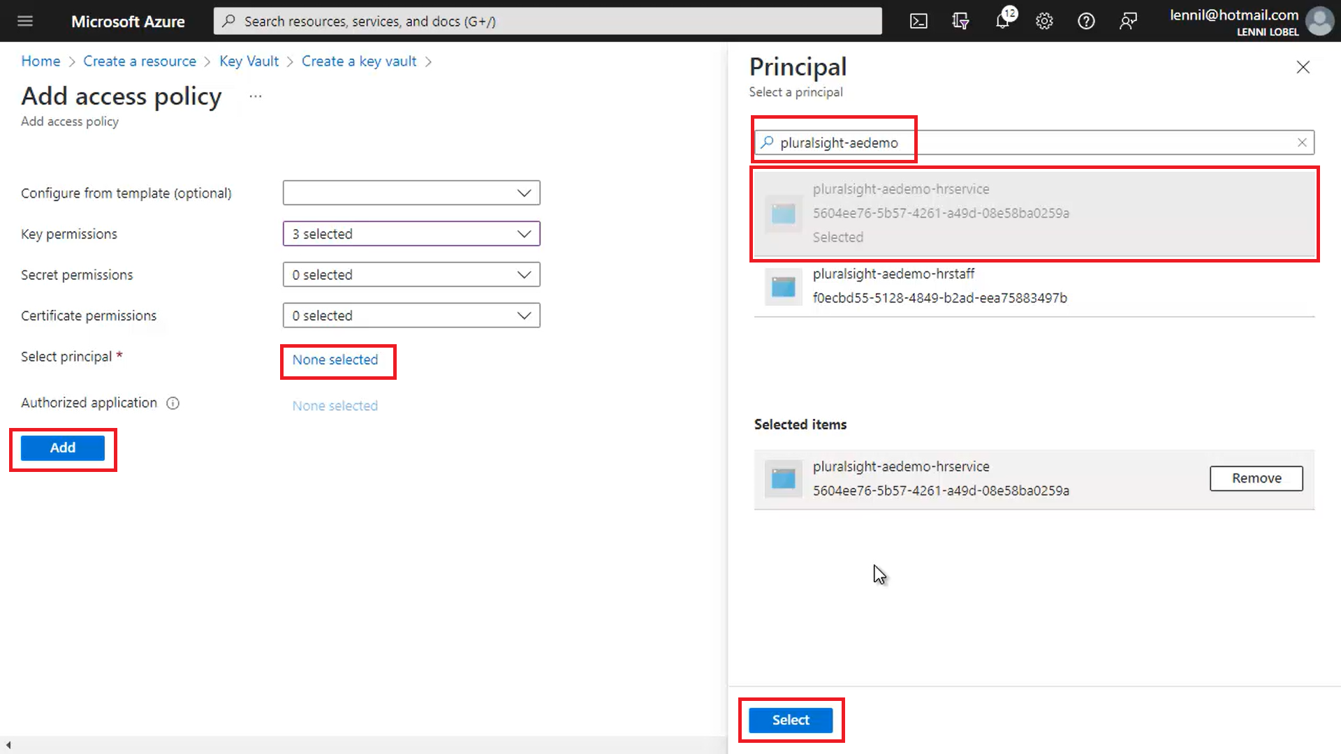
Each policy can be granted a variety of permission, and for our scenario, we need three permissions in particular. So click the Key permissions dropdown and check the Get, Unwrap Key, and Sign permissions:
And then choose the principal, which is the app registration.
Click the None selected link, and then filter the list this down to pluralsight-aedemo, and you’ll find the two app registrations that we created starting with that name, which are the two that we need. For this access policy we’ll choose the pluralsight-aedemo-hrservice app registration, and then we’ll create a second access policy for this key vault that points to the pluralsight-aedemo-hrstaff app registration.
Click Select to choose the app registration, and then click Add to create the access policy:
Now repeat for the second access policy:
Click Add Access Policy
Check the three key permissions for Get, Unwrap Key, and Sign
Choose the principal (app registration) pluralsight-aedemo-hrstaff
Click Add
And now, here are the two access policies we just created for both HR applications:
Again, this means that both applications can access this key vault, which is where we’ll store the customer-managed key for encrypting and decrypting the salary property in each document.
So now click Review & Create, and then Create, and just a few moments later, we have our new key vault:
Now let’s create the key itself. Click on Keys, and then Generate/Import:
This key is for the salary property, so let’s name it hr-salary-cmk, for customer-managed-key. All the other defaults are fine, so just click Create.
And we’ve got our new CMK. We’ll need an ID for this CMK when we create our employees container, so click to drill in:
Now copy its Key identifier, and paste that into Notepad:
Finally, repeat this process for the second key vault.
Create a Resource, search for key vault, and click Create.
Name the new key valut hr-ssn-kv
Click Next for the access policy, only this time create just one for the HR Service application, and not the HR Staff application, which should not be able to access the social security number property.
Check the key permissions Get, Unwrap key, and Sign.
For the principal, select the app registration for the HR Service application – pluralsight-aedemo-hrservice.
Click Add to create the access policy
Click Review and Create, and Create to create the second key vault.
Click Keys, Generate/Import
Name the new key hr-ssn-cmk and click Create.
Click into the CMK to copy its key identifier and paste it into Notepad
All our work is done in the Azure portal. At this point, your Notepad document should contain:
Azure AD directory ID
Two HR application client IDs
Two HR application secrets
Two customer-managed key IDs
Save this document now. It will be needed when we build the two client applications in my next post.
In my previous post, I explained how server-side encryption works in Cosmos DB. You can rely on the server-side encryption that’s built into the service, and can also add another layer of encryption using customer-managed keys so that even Microsoft cannot decrypt your data without access to your own encryption keys.
Beyond server-side encryption, Cosmos DB supports client-side encryption – a feature that’s also known as Always Encrypted. In this post, I’ll introduce client-side encryption at a high level. My next two posts will then dig into the process of how to configure this feature, and use it in your .NET applications.
Because your data is always encrypted only on the server-side, enabling client-side encryption as well means that your data is truly always encrypted, even as it flows into and out of your client. Let’s start with a quick review of server-side encryption, and then see how client-side encryption works to achieve data that’s always encrypted.
Here’s an application that generates some data, and on the client-side that data is not encrypted:
When the client sends the data across the internet to the server-side, it gets encrypted in-flight using SSL, and then once it crosses that boundary, Cosmos DB encrypts the data as I explained in my previous post – meaning that it gets encrypted using a Microsoft-managed encryption key, and then optionally double-encrypted using a customer-managed key. It then continues to make its way across the network, where it remains encrypted in flight until it reaches your Cosmos DB account, where it’s stored in the database, encrypted at rest. And the return trip is similar; the data is encrypted in flight on the way back, across the wire to the client, where it arrives decrypted for the client application to consume.
So you can see how – on the client side – the data is not encrypted. In fact, the client will never see the encrypted state of the data because the encryption is only happening on the server-side. So essentially every client is able to see all the data being returned from the server.
With client-side encryption, we rely on the .NET SDK to handle encryption from right inside your application, where the application itself requires access to customer-managed encryption keys that are never, ever, exposed to the Cosmos DB service.
This process is completely transparent, so as soon as the application generates any data, the SDK immediately encrypts it before it ever gets to leave the application. Furthermore, this process is capable of encrypting only the most sensitive properties in your document, without necessarily having to encrypt the entire document. So properties like credit card numbers and passwords for example are encrypted on the client-side, from within your application, automatically by the SDK, right inside the document that your application is creating for the database.
The document then continues on to the server where now, it gets at least one additional layer of encryption using a Microsoft-managed key, and possibly one more layer of encryption if you’ve supplied a customer-managed key for server-side encryption. But even if you peel those encryption layers off on the server-side, the properties encrypted using your customer-managed key on the client side can never be revealed. So the data gets written to Cosmos DB, where ultimately, Cosmos DB – and that means Microsoft itself, is utterly incapable of reading those properties that were encrypted on the client. And that’s because the CMK used for client-side encryption is never revealed anywhere outside the client application.
Likewise, when returning data back to the client, those protected properties remain encrypted throughout the flight back to the application. Again, assuming the application has been granted access to the client-side customer-managed key, the SDK seamlessly decrypts the protected properties for the application.
Stay tuned for my next post, where I’ll show you how to configure client-side encryption for Cosmos DB using the Azure portal.
Encryption is an important way to keep you data secured. Cosmos DB has server-side encryption built into to the service, so that on the server-side of things, your data is always encrypted – both in flight – as it travels the network, and at rest – when it’s written to disk. As I said, this functionality is built-in, and there’s simply no way to disable this encryption.
One nice part of this feature is that Microsoft creates and manages the keys used for server-side encryption, so there are no extra steps you need to take in order to make this work. Your data is simply encrypted on the server-side using encryption keys managed entirely by Microsoft. As part of this management, Microsoft applies the usual best practices, and protects these keys with a security life cycle that includes rotating keys on a regular basis.
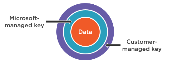
In addition, customer-managed encryption keys are also supported, so that you can use your own encryption keys. This adds another layer of encryption, on top of the encryption based on Microsoft-managed keys that, again, can never be disabled. That said, using customer-managed keys is generally discouraged, unless you are absolutely obliged by regulatory compliance guidelines mandated by your industry. And the reason for this is simple; because then you become responsible for managing those keys, and that’s a huge responsibility. Now you need to maintain and rotate encryption keys yourself, and if you should lose a key, then you lose access to all your data, and Microsoft will not be able to help you recover it. And another relatively minor consideration is that you’re going to incur a slight increase in RU charges when using customer-managed keys, because of the additional CPU overhead needed to encrypt your data with them.
So again, using customer-managed keys does not disable the default behavior; your data still gets encrypted using a Microsoft managed key. The result is double-encryption, where that encrypted data is then encrypted again using your own key that you supply.
Currently, you can only configure your account to use customer-managed keys when you’re creating the account; they cannot be enabled on an existing account. So here in the portal, during the process of creating a new account, the Encryption tab lets you set it up.
The default is to use a service-managed key – that is, the one provided and managed by Microsoft, but you can also choose to use a customer-managed key. And when you make this choice, the portal prompts you for the Key URI, and that’s simply the path to your own key that you’ve got stored in your own Azure key vault.
So you see that it’s pretty simple to configure your Cosmos DB account to encrypt your data using your own encryption key that you have in Azure Key Vault.
Beyond server-side encryption, Cosmos DB supports client-side encryption – a feature that’s also known as Always Encrypted. Because your data is always encrypted on the server-side, enabling client-side encryption as well means that your data is truly always encrypted, even as it flows into and out of your client. So stay tuned for my next post where we’ll dive into client-side encryption with Always Encrypted.
Network security is your first line of defense against unauthorized access to your Cosmos DB account. Before a client can even attempt to authenticate against your account, it needs to be able to establish a physical network connection to it.
Now Cosmos DB is a cloud database service on Azure, and Azure is a public cloud, so by default, a new Cosmos DB account can be accessed from anywhere on the internet. While this is very convenient when you’re getting started, such exposure is often unacceptable for sensitive mission-critical databases running in production environments.
And so, there are several ways for you to lock down network access to your Cosmos DB account.
IP Firewall
First, you can use the IP firewall which is both simple and effective. This works very much like firewalls that you find in other systems, where you maintain a list of approved IP addresses, which could be individual addresses, or address ranges. Network traffic from IP addresses that are not approved, get blocked from the firewall; while traffic from approved addresses are allowed to pass through the firewall, and reach your account by its public IP address.
So here I’ve got my Cosmos DB account, which can be reached by its public endpoint, and that’s a public IP address on the internet. And we’ve got two clients hanging out on the internet, each on their own public IP address. Now by default, both clients can reach our account, but if we enable the IP firewall, then we can add the IP address for the first one, with the IP address ending in 140, so that incoming traffic from that client is allowed access to the account’s public endpoint. Meanwhile, since we haven’t added the IP address for the second client ending in 150, that client gets blocked and can’t access the account.
In the Azure Portal, head on over to Firewall and Virtual Networks, where by default, any client can access the account. But if you choose selected networks, then you can configure the firewall.
There are actually two sections to this page, and right now we’re focused on the bottom section, Firewall. Here you can add IP addresses, or IP address ranges, one at a time, for approved clients, while clients from all other IP addresses are unapproved and get blocked by the firewall.
To make it easier to connect through the firewall from you own local machine, you can click on Add My Current IP, where the portal automatically detects your local machine’s IP address. You can see I’ve done this in the previous screenshot, where my local IP address has been added to the firewall as an approved client.
Also take note of the bottom two checkboxes for exceptions. First, you may reluctantly want to select the first checkbox, which accepts connections from within public Azure data centers. You would only do this if you need access to your account from a client running on Azure that can’t share its IP address or IP address range. And these can be VMs, functions, app services; any kind of client. Again, this is why you want to be cautious with this checkbox, because selecting it would accept connections from any other customer that’s running a VM.
The second checkbox, which is selected by default, makes sure that the account can always be reached by the Cosmos DB portal IPs; so you’ll want to keep this setting if you want to use portal features – notably the Data Explorer, with your account.
When you click Save, be prepared to wait a bit for the changes to take effect. With the distributed nature of the Cosmos DB service, it can take up to 15 minutes for the configuration to propagate, although it usually less time than that. And then, the firewall is enabled, blocking network traffic from all clients except my local machine.
VNet Through Service Endpoint
Using the IP firewall is the most basic way to configure access control, but it does carry the burden of having to know the IP addresses of all your approved clients, and maintaining that list.
With an Azure virtual network, or a VNet, you can secure network access to all clients hosted within that VNet, without knowing or caring what those client IP addresses are. You just approve one or more VNets, and access to your account’s public endpoint is granted only to clients hosted by those VNets. Like the IP firewall, all other clients from outside approved VNets are blocked from your account’s public endpoint.
So once again, we have our Cosmos DB account with its public endpoint. And we’ve got a number of clients that need to access our account. But rather than approve each of them to the firewall individually by their respective IP addresses, we simply host them all on the same virtual network. Then, when we approve this VNet for our account, that creates a service endpoint which allows access to our account only from clients that the VNet is hosting.
If you run an NSLookup to the fully qualified domain name for your account, from within the VNet, you can see that this resolves to a public IP address, for your account’s public endpoint:
You can approve individual VNets from the top section of the same page we were using to configure the IP firewall, where you use these links to choose a new or existing vnet.
Here I’ve added an existing VNet which I’ve named cosmos-demos-rg-vnet, and you can see the VNet is added as approved. Also notice that you can mix-and-match, combining VNet access with the IP firewall, so you can list both approved IP addresses and approved VNets on this one page in the Azure portal, like you see above.
VNet Through Private Endpoint
VNet access using service endpoints is very convenient, but there’s still a potential security risk from within the VNet. Because as I just showed you, the Cosmos DB account is still being accessed by its public endpoint through the VNet’s service endpoint, and that means that the VNet itself can connect to the public internet. So a user that’s authorized to access the VNet could, theoretically, connect to your Cosmos DB account from inside the VNet, and then export it out to anywhere on the public internet.
This security concern known as exfiltration, and can be addressed using your third option, VNet access using private endpoints.
This is conceptually similar to using VNets with service endpoints like we just saw, where only approved VNets can access your account. However now, the VNet itself has no connection to the public internet. And so, when you enable private endpoints, you’ll see that your Cosmos DB account itself is accessible only through private IP addresses that are local to the VNet. This essentially brings your Cosmos DB account into the scope of your VNet.
So again here’s our Cosmos DB account which, technically still has a public endpoint, but that public endpoint is now completely blocked to public internet traffic. Then we’ve got our clients that, like before, all belong to the same VNet that we’ve approved for the account. However, now the VNet has no public internet access, and communicates with your Cosmos DB account using a private IP address accessible only via the private endpoint that you create just for this VNet.
So if you run NSLookup from within a VNet secured with a private endpoint, you can see that your account’s fully qualified domain name now resolves to a private IP address. And so, there’s simply no way for a malicious user that may be authorized for access to the VNet, to exfiltrate data from your account out to the public internet.
It’s fairly straightforward to configure a private endpoint for your VNet. Start by clicking to open the Private Endpoint Connections blade, and then to create a new one. This is actually a new resource that you’re adding to he same resource group as the VNet that you’re securing.
Just give your new private endpoint a name, and click Next to open the Resource tab.
Here you select the resource type, which is Microsoft Azure Cosmos DB slash Database Accounts, and the resource itself, which is the Cosmos DB account you are connecting to with this new private endpoint. Then there’s the target sub-resource, which is just the API that you’ve chosen for the account, and that’s the SQL API in this case.
Then click Next for the Virtual Network tab, where you can choose the VNet and its subnet for the new private endpoint.
Notice that Private DNS Integration option is turned on by default, and this is what transparently maps your account’s fully qualified domain name to a private IP address. So, really without you having to do anything different in terms of how you work with your Cosmos DB account, this makes the account accessible only from the private endpoint in this VNet, which itself is accessible only through private IP addresses, and no access to the public internet.
And that’s pretty much it. Of course, you can assign tags to the private endpoint just like with any Azure resource, and then just click Create. It takes a few moments for Azure to create and deploy the new private endpoint, and then you’re done.
Summary
This post examined three different ways to secure network access to your Cosmos DB account. You can approve IP addresses and IP address ranges with the IP firewall, or approve specific virtual networks using service endpoints. Both of these options carry the risk of exfiltration, since the Cosmos DB account is still accessible via its public endpoint. However, you can eliminate that risk using your third option, which is to use private endpoints with virtual networks that are completely isolated from the public internet.
Protecting your data is critical, and Cosmos DB goes a long way to provide redundancy so you get continuous uptime in the face of hardware failures, or even if an entire region suffers an outage. But there are other bad things that can happen too – notably, any form of accidental corruption or deletion of data – and that’s why Cosmos DB has comprehensive backup and restore features.
There are actually two versions of this feature you can choose from; periodic backups, and continuous backups.
Periodic backups are the default, and they are both automatic and free. Meaning that, at regular intervals, Cosmos DB takes a backup of your entire account, and saves it to Azure Blob Storage, always retaining at least the two most recent backups. This occurs without absolutely zero impact on database performance, and with no additional charges to your Azure bill.
Backups are retained for 8 hours by default, but you can request retention for up to 30 days if you need. However, this is where you begin to incur charges for periodic backups, since the longer you retain backups, the more snapshot copies need to be kept in Azure Blob Storage – and only the first two are free. So depending on how frequently you set the backup interval, and how long you request backup retention – Cosmos DB may keep anywhere from 2 to 720 snapshots in Azure Blob Storage available for restore.
In the unfortunate event that you do need a restore, you do that by opening a support ticket in the portal, and I’ll show you what that looks like in a moment.
Your other option is to use continuous backup, which does cost extra, but lets you perform a point-in-time restore – meaning, you can restore your data as it was at any point in time within the past 30 days, and you don’t deal with intervals, snapshots, and retention.
Continuous backup carries a few limitations – at least right now, you can use it only with the SQL and Mongo DB APIs. And while it does work with geo-replicated accounts, it doesn’t work if you’ve enabled multi-master; that is, multi-region writes – it needs to be a single-write region account.
If you need to restore data to an account using continuous backups, you can do it yourself right inside the Azure portal. You don’t need to open a ticket with the support team, like you do with periodic backups.
Periodic Backups
As I said, periodic backup is the default backup mode, and it can be configured at the same time you create a new Cosmos DB account. Here in the Backup Policy tab for a new account, we see periodic backup is selected by default, to automatically take backups every 4 hours (that’s 240 minutes) and retain them for 8 hours. This results in 2 copies always being retained at any given time.
Also notice that, by default, you get geo-redundant backup storage, which adds yet another layer of data protection. So – even for single-region accounts – your backups will be written to two regions; the region where the account resides, and the regional pair associated with that region. All backups are encrypted at rest, and in-flight as well, as they get transferred for geo-redundancy to the regional pair, using a secure non-public network.
Once the account is created, you can navigate over to the Backup and Restore blade and reconfigure the periodic backups. For example, I can go ahead and change the interval from four hours, to be every hour.
Increasing the frequency for the same retention period of 8 hours results in 8 copies being retained, and so we see a message telling us that we’re incurring an extra charge for storage, since only the first 2 copies are free. Currently, that charge is fifteen cents a month per gigabyte of backup storage, though charges can vary by region.
Now if I bump up the retention period from 8 hours to 720, which is 30 days now I’m retaining 720 backup copies, since we’re taking one backup an hour and retaining them for 720 hours.
To restore from a periodic backup, you need to open a support ticket by scrolling all the way down on the left and choosing New Support Request. For basic information, you need to type a brief summary description, and indicate that type of problem you need help with. For example, I’ll just say Restore from backup for the summary. Then when I choose Backup and Restore as the Problem Type, I can then choose Restore Data For My Account as the Problem Subtype.
Then click Next to move on to the Solutions tab.
There’s no input on this tab, it just has a lot of useful information to read about restoring your data. For example, it recommends increasing the retention to within 8 of the desired restore point, in order to give the Cosmos DB team enough time to restore your account – among other things to consider for the restore. It also explains how long you can expect to wait for the restore, which – while there’s no guarantee – is roughly four hours to restore about 500 GB of data.
Next you’re on the Details tab, where you supply the specifics. Like when the problem started, and whether you need to restore deleted or corrupted data. As you input this form, you can indicate whether you need to restore the entire account, or only certain databases and containers. Then scrolling down some, you can put in your contact info and how you prefer to be contacted.
Then click Next to review your support request.
Finally, click Create to open the ticket to restore your data.
Continuous Backup
Now lets have a look at continuous backups, which work quite a bit differently than periodic backups.
Here on the Backup Policy tab, when you’re creating a new account, you can just click Continuous, and you’ll get continuous backups for the new account.
And there again we get a message about the additional charges that we’ll incur for this feature. Currently, the charge for continuous backup storage is 25 cents a month per gigabyte, and for geo-replicated accounts, that gets multiplied by the number of regions in the account. There’s also a charge for if and when you need to perform a point-in-time restore, and that’s currently 19 cents per gigabyte of restored data. And again, this can vary by region, so it’s always best to check the Cosmos DB Pricing page for accurate charges.
If you don’t enable continuous backups at account creation time, you’ll get periodic backups instead. And then, you can head over to the Features blade showing that Continuous Backup is Off.
Simply click to enable it; though note that once continuous backups are turned on for the account, you cannot switch back to using periodic backups.
Now that continuous backups are enabled, the Backup and Restore blade gets replaced by the Point-In-Time Restore blade.
This blade lets you restore from the continuous backup yourself, without opening a support ticket with the Cosmos DB team. Just plug in any desired point-in-time for the restore within the past 30 days. You can also click the link on Need help with identifying restore point? to open the event feed, which shows a chronological display of all operations to help you determine that the exact time should be.
Then you pick the location where the account gets restored, which needs to be a location where the account existed at the specified point-in-time. Then you get to choose whether to restore the entire account, or only specific databases and containers, and finally, the resource group and name for a new account where all the data gets restored to.
Then click Submit, and you’ve kicked off the restore.
Summary
Recovering from backups is something we all like to avoid. But when it becomes necessary, it’s good to know that Cosmos DB has you covered with your choice of periodic or continuous backups. So you can sleep easy knowing that you’re protected, if you ever need to recover from accidental data corruption or deletion.
In this blog post, I’ll show you how to easily and effectively implement time zone support, with Daylight Savings Time (DST) awareness, in your web applications (Angular with ASP.NET Core)
Historically, these issues have always stuck a thorn in the side of application development. Even if all your users are in the same time zone, Daylight Savings Time (DST) will still pose a difficult challenge (if the time zone supports DST). Because even within a single time zone, the difference between 8:00am one day and 8:00am the next day will actually be 23 hours or 25 hours (depending on whether DST had started or ended overnight in between), and not 24 hours like it is in all other instances throughout the year.
When your application is storing and retrieving historical date/time values, absolute precision is critical. There can be no ambiguity around the exact moment an entry was recorded in the system, regardless of the local time zone or DST status at any tier; the client (browser), application (web service), or database server.
General consensus therefore is to always store date/time values in the database as UTC (coordinated universal time), a zero-offset value that never uses DST. Likewise, all date/time manipulation performed by the application tier in the web service is all in UTC. By treating all date/time values as UTC on the back end (from the API endpoint through the database persistence layer), your application is accurately recording the precise moment that an event occurs, regardless of the time zone or DST status at the various tiers of the running application.
Note: UTC is often conflated with GMT (Greenwich Mean Time), since they both represent a +00:00 hour/minute offset. However, GMT is a time zone that happens to align with UTC, while UTC is a time standard for the +00:00 offset that never uses DST. Unlike UTC, some of the countries that use GMT switch to different time zones during their DST period.
Note: SQL Server 2008 introduced the datetimeoffset data type (also supported in Azure SQL Database). This data type stores date/time values as UTC internally, but also embeds the local time zone offset to UTC in each datetimeoffset instance. Thus, date/time values appear to get stored and retrieved as local times with different UTC offsets, while under the covers, it’s still all UTC (so sorting and comparisons work as you’d expect). This sounds great, but unfortunately, the datetimeoffset data type is not recommended for two reasons; it lacks .NET support (it is not a CLS-compliant data type), and it is not DST-aware. This is why, for example, the SQL Server temporal feature (offering point-in-time access to any table) uses the datetime2 data type to persist date/time values that are all stored in UTC.
Once you store all your date/time values as UTC, you have accurate data on the back end. But now, how do you adapt to the local user’s time zone and DST status? Users will want to enter and view data in their local time zone, with DST adjusted based on that time zone. Or, you might want to configure your application with a designated “site” time zone for all users regardless of their location. In either scenario, you need to translate all date/time values that are received in client requests from a non-UTC time zone that may or may not be respecting DST at the moment, into UTC for the database. Likewise, you need to translate all date/time values in the responses that are returned to the client from UTC to their local time zone and current DST status.
Of course, it’s possible to perform these conversions in your application, by including the current local time zone offset appended as part of the ISO-formatted value in each API request; for example, 2021-02-05T08:00:00-05:00, where -05:00 represents the five hour offset for Eastern Standard Time (EST) here in New York. Unfortunately, here are three complications with this approach.
The first problem is that it only works for current points in time. For example, in July, EST respects DST, and so the offset is only four hours from UTC, not five; for example, 2021-07-05T08:00:00-04:00. This translates fine, since the current offset in July is actually four hours and not five. But if, in July, the user is searching for 8:00am on some past date in February, then the value 2021-02-05T08:00:00-04:00 is off by an hour, which of course yields incorrect results. This means that you really need to know the actual time zone itself, not just the current offset.
Second, resolving DST remains a problem that’s not easily solved on the client. Because some time zones don’t respect DST at all, and those that do respect DST all switch to and from DST at different dates from year to year.
And last, the onus is then on every developer to include code that converts from local to UTC in the request, and from UTC to local in the response. Every date/time value instance must be accounted for in both directions, so it is all too easy for a developer to miss a spot here and there. The result, of course, is a system that’s both difficult to maintain and error prone.
The solution explained here addresses all these concerns by leveraging middleware in ASP.NET Core. This is a feature that allows you to intercept all incoming requests and modify the request content after it leaves the client, but before it reaches your endpoint. Likewise, you can intercept all outgoing responses and modify the response content before it gets returned to the client, but after you have finished processing the request.
Thus, we will write some middleware that discovers every date/time value found in the JSON body (or query string parameters in the URI) associated with the request, and converts it to UTC. Likewise, it discovers every date/time value found in the JSON body associated with the response, and converts it to the user’s local time zone. Of course, to properly perform the conversions with DST awareness, the server needs to know the local time zone (not just the current time zone offset). This is the only responsibility that falls on the client; it needs to inform the server what the local time zone is with every request. All the rest of the heavy processing happens in the middleware on the server.
Write an Angular Interceptor
This is fairly straightforward; we want to inject the local time zone into the HTTP header of every API request issued by our Angular client:
import { HttpEvent, HttpHandler, HttpInterceptor, HttpRequest } from "@angular/common/http";
import { Injectable } from "@angular/core";
import { Observable } from "rxjs";

@Injectable()
export class TimeZoneInterceptorService implements HttpInterceptor {
  public intercept(req: HttpRequest<any>, next: HttpHandler): Observable<HttpEvent<any>> {
    const modifiedReq = req.clone({
      headers: req.headers.set('MyApp-Local-Time-Zone-Iana', Intl.DateTimeFormat().resolvedOptions().timeZone),
    });
    return next.handle(modifiedReq);
  }
}
This class implements the HttpInterceptor interface provided by Angular, which requires that you supply an intercept method. It receives the incoming request in req and modifies it by cloning it while adding a new header named MyApp-Local-Time-Zone-Iana with the value returned by Intl.DateTimeFormat().resolvedOptions().timeZone. That mouthful simply returns the client’s local time zone in IANA format, one of several different standards for expressing time zones. For example, here in New York, the IANA-formatted time zone is America/New_York.
Configure the Middleware Class
In Starup.cs, add code to the Configure method to plug in a class that we’ll call RequestResponseTimeZoneConverter. As the name implies, this class will convert incoming and outgoing date/time values to and from UTC and the client’s local time zone:
Our middleware class needs to implement the Invoke method that will fire for each request, which can process each incoming request and outgoing response. Start with the namespace imports and class definition like so:
using Microsoft.AspNetCore.Http;
using Microsoft.AspNetCore.Http.Extensions;
using Microsoft.Extensions.Options;
using Microsoft.Extensions.Primitives;
using Newtonsoft.Json;
using OregonLC.Shared;
using OregonLC.Shared.Extensions;
using System;
using System.Collections.Generic;
using System.IO;
using System.Linq;
using System.Net.Http;
using System.Text;
using System.Threading.Tasks;
using TimeZoneConverter;

namespace TimeZoneDemo
{
  public class RequestResponseTimeZoneConverter
  {
    private readonly AppConfig _appConfig;
    private readonly RequestDelegate _next;

    public RequestResponseTimeZoneConverter(
        IOptions<AppConfig> appConfig,
        RequestDelegate next)
    {
      this._appConfig = appConfig.Value;
      this._next = next;
    }

  }
}
Notice that we’re also injecting IOptions<AppConfig> for a strongly typed configuration object based on appsettings.json, where we define settings that can influence the time zone conversion behavior of our middleware.
Now implement the Invoke method:
public async Task Invoke(HttpContext context)
{
  // Request content and parameters won't be modified if disableTimeZoneConversion=true is specified
  // as a query string parameter in the URI
  var disableConversion =
    context.Request.Query.ContainsKey("disableTimeZoneConversion") &&
    context.Request.Query["disableTimeZoneConversion"] == "true";

  // Get the local time zone for UTC conversion
  var localTimeZone = this.GetLocalTimeZone(context);

  // If conversion isn't disabled, and the local time zone can be detected (and isn't UTC),
  // modify the request content (convert local to UTC)
  if (!disableConversion && localTimeZone != null && localTimeZone.Id != "UTC")
  {
    // Modify the date/time request parameters in the URI
    this.ModifyRequestParameters(context, localTimeZone);

    // Don't modify the request content unless the Content-Type is application/json
    var isJsonContent =
      context.Request.Headers.ContainsKey("Content-Type") &&
      context.Request.Headers["Content-Type"] == "application/json";

    if (isJsonContent)
    {
      // Modify the date/time properties in the request content
      await this.ModifyRequestContent(context, localTimeZone);
    }
  }

  // Prepare for modifying the response body
  var responseStream = context.Response.Body;
  var modifiedResponseStream = new MemoryStream();
  context.Response.Body = modifiedResponseStream;

  try
  {
    await this._next(context).ConfigureAwait(false);
  }
  finally
  {
    context.Response.Body = responseStream;
  }

  // Modify the response content (convert UTC to local)
  modifiedResponseStream = this.ModifyResponseContent(context, disableConversion, localTimeZone, modifiedResponseStream);
  await modifiedResponseStream.CopyToAsync(responseStream).ConfigureAwait(false);
}

private TimeZoneInfo GetLocalTimeZone(HttpContext context)
{
  // If the app config doesn't permit multiple time zones, then treat every user as if
  // they were in the same "site" time zone
  if (!this._appConfig.SupportMultipleTimeZones)
  {
    return TimeZoneInfo.FindSystemTimeZoneById(this._appConfig.SiteTimeZoneId);
  }

  // If the request headers include the user's local time zone (IANA name, injected by client-side HTTP interceptor),
  // use that time zone
  if (context.Request.Headers.TryGetValue("MyApp-Local-Time-Zone-Iana", out StringValues localTimeZoneIana))
  {
    return TZConvert.GetTimeZoneInfo(localTimeZoneIana);
  }

  // The app config permits multiple time zones, but the user request doesn't specify the time zone
  return null;
}
The code is heavily commented to make it self-describing, so I’ll just call out the main aspects. We’ll allow the client to disable time zone conversion on a per-request basis, by supplying disableTimeZoneConversion=true as a query string parameter. We then call GetLocalTimeZone, which first checks our app configuration to see if the server application wants to support multiple time zones, or a consistent “site” time zone for all clients. So if we see that SupportMultipleTimeZones is false, then we ignore the client’s local time zone injected by our Angular interceptor, and use the same “site” time zone for all users instead, as defined by SiteTimeZoneId in the app configuration.
Otherwise, we get the client’s local time zone by retrieving the MyApp-Local-Time-Zone-Iana custom HTTP header injected by the interceptor. Because .NET requires the time zone in Windows format, we use the TZConvert.GetTimeZoneInfo method (available by installing the TimeZoneConverter NuGet package) to convert from the IANA format supplied by the client into a Windows TimeZoneInfo object. For example, it will convert America/New_York to (UTC-05:00) Eastern Time (US & Canada).
Then, as long as this client request hasn’t explicitly disabled time conversion, and the client’s local time zone itself isn’t UTC (meaning no conversion is necessary anyway), we call ModifyRequestParameters to convert all date/time values supplied as query string parameters in the request URI to UTC. And then, after verifying that the request content being posted to our API is, in fact, a JSON payload, we call ModifyRequestContent to convert all date/time values inside that JSON content to UTC as well.
Before allowing the request to process, we capture the current response stream in case of exception, and set the response body to a new stream for our modified response. We then call this._next to invoke the request, with exception handling in place to use the original response stream in case an error occurs processing the request. Otherwise, we call ModifyResponseContent to convert all date/time values inside the JSON response payload from UTC back to the client’s local time zone.
Modify the Request Query String Parameters (local to UTC)
Now add the ModifyRequestParameters method to handle query string parameters:
private void ModifyRequestParameters(HttpContext context, TimeZoneInfo localTimeZone)
{
  // Get all the query parameters from the URI
  var queryParameters = context.Request.Query
    .SelectMany(kvp =>
      kvp.Value, (col, value) =>
        new KeyValuePair<string, string>(col.Key, value))
    .ToList();

  // Nothing to do if there aren't any
  if (queryParameters.Count == 0)
  {
    return;
  }

  // Build a new list of query parameters, converting date/time values
  var modifiedQueryParameters = new List<KeyValuePair<string, string>>();

  var modified = false;
  foreach (var item in queryParameters)
  {
    var value = item.Value;
    if (value.FromDateTimeIsoString(out DateTime local))
    {
      var utc = TimeZoneInfo.ConvertTimeToUtc(local, localTimeZone);
      value = utc.ToDateTimeIsoString();
      var modifiedQueryParameter = new KeyValuePair<string, string>(item.Key, value);
      modifiedQueryParameters.Add(modifiedQueryParameter);
      modified = true;
    }
    else
    {
      var unmodifiedQueryParameter = new KeyValuePair<string, string>(item.Key, value);
      modifiedQueryParameters.Add(unmodifiedQueryParameter);
    }
  }

  if (modified)
  {
    var qb = new QueryBuilder(modifiedQueryParameters);
    context.Request.QueryString = qb.ToQueryString();
  }
}
We first obtain all the query parameters from the request URI, from which we build a new list of parameters with any date/time values converted from local to UTC. This code relies on the two extension methods FromDateTimeIsoString and ToDateTimeIsoString to parse to and from ISO-formatted date/time strings and native .NET DateTime types:
public static bool FromDateTimeIsoString(this string value, out DateTime dateTime)
{
  if (
      (value.Length == 16 || (value.Length == 19 && value[16] == ':')) &&
      value[4] == '-' &&
      value[7] == '-' &&
      value[10] == 'T' &&
      value[13] == ':' &&
      DateTime.TryParse(value, out DateTime parsedDateTime)  // calls DateTime.TryParse only after passing the smell test
     )
  {
    dateTime = parsedDateTime;
    return true;
  }

  dateTime = DateTime.MinValue;
  return false;
}

public static string ToDateTimeIsoString(this DateTime value) =>
  value.ToString("yyyy-MM-ddTHH:mm:ss");
Modify the Request Body Content (local to UTC)
Next add the ModifyRequestContent method to handle the JSON request payload:
private async Task<TimeZoneInfo> ModifyRequestContent(HttpContext context, TimeZoneInfo localTimeZone)
{
  // Read the request content from the request body stream; if it's a JSON object, we'll process it
  var requestStream = context.Request.Body;
  var originalRequestContent = await new StreamReader(requestStream).ReadToEndAsync();

  // Try to get the JSON object from the request content
  var jobj = originalRequestContent.TryDeserializeToJToken();

  // If the request content is a JSON object, convert all of it's date/time properties from local time to UTC
  var modified = false;
  if (jobj != null)
  {
    modified = jobj.ConvertLocalToUtc(localTimeZone);
  }

  if (modified)
  {
    // Replace the stream with the updated request content
    var json = JsonConvert.SerializeObject(jobj);
    var requestContent = new StringContent(json, Encoding.UTF8, "application/json");
    requestStream = await requestContent.ReadAsStreamAsync();
  }
  else
  {
    // Replace the stream with the original request content
    requestStream = new MemoryStream(Encoding.UTF8.GetBytes(originalRequestContent));
  }

  // Replace the request body stream
  context.Request.Body = requestStream;

  // Return the time zone info for the reverse conversion on the response
  return localTimeZone;
}
We first try to deserialize the JSON, and if that succeeds, we convert all of its date/time properties from local to UTC. We then replace the original stream with the updated content, unless we detect that there were no date/time properties at all in the request, in which case we continue with the original stream.
Again, we have some extension methods here to help out, which are TryDeserializeToJToken and ConvertLocalToUtc:
public static JToken TryDeserializeToJToken(this string json)
{
  if (json == null || (!json.StartsWith("[") && !json.StartsWith("{")))
  {
    return null;
  }

  // Try to get the JSON object from the request content
  var jToken = default(JToken);
  try
  {
    jToken = JsonConvert.DeserializeObject<JToken>(json);
  }
  catch
  {
    // Ignore the exception, returning null to indicate bad JSON
  }

  return jToken;
}

public static bool ConvertLocalToUtc(this JToken token, TimeZoneInfo localTimeZone, bool wasModified = false)
{
  var modified = wasModified;
  if (token.Type == JTokenType.Object)
  {
    modified = ConvertLocalToUtcForObject(token, localTimeZone, wasModified, modified);
  }
  else if (token.Type == JTokenType.Array)
  {
    modified = ConvertLocalToUtcForArray(token, localTimeZone, wasModified, modified);
  }
  return modified;
}

private static bool ConvertLocalToUtcForObject(JToken token, TimeZoneInfo localTimeZone, bool wasModified, bool modified)
{
  foreach (var prop in token.Children<JProperty>())
  {
    var child = prop.Value;
    if (child is JValue jValue)
    {
      var value = ParseJsonValueForDateTime(jValue.Value);
      if (value is DateTime)
      {
        var local = (DateTime)value;
        var utc = TimeZoneInfo.ConvertTimeToUtc(local, localTimeZone);
        jValue.Value = utc;
        modified = true;
      }
    }
    else if (child.HasValues)
    {
      modified = child.ConvertLocalToUtc(localTimeZone, wasModified) || modified;
    }
  }

  return modified;
}

private static bool ConvertLocalToUtcForArray(JToken token, TimeZoneInfo localTimeZone, bool wasModified, bool modified)
{
  foreach (var item in token.Children())
  {
    var child = item;
    if (child.HasValues)
    {
      modified = child.ConvertLocalToUtc(localTimeZone, wasModified) || modified;
    }
  }

  return modified;
}
Modify the Response Body Content (UTC to local)
The last part is the ModifyResponseContent to handle the response, which converts date/time values from UTC back to the client’s local time zone:
private MemoryStream ModifyResponseContent(
  HttpContext context,
  bool disableConversion,
  TimeZoneInfo localTimeZone,
  MemoryStream responseStream)
{
  // Rewind the unmodified response stream
  responseStream.Position = 0;
  var modified = false;

  // Will capture the unmodified response for time zone conversion
  var responseContent = default(string);

  // Only attempt to modify the response if time zone conversion is not disabled
  // and we have a local time zone that was used to modify the request
  if (!disableConversion && localTimeZone != null)
  {
    // Capture the unmodified response
    responseContent = new StreamReader(responseStream).ReadToEnd();

    // Try to get the JSON object from the response content
    var jobj = responseContent.TryDeserializeToJToken();

    // If the response content is a JSON object, convert all of it's date/time properties from local time to UTC
    if (jobj != null && jobj.ConvertUtcToLocal(localTimeZone))
    {
      responseContent = JsonConvert.SerializeObject(jobj);
      modified = true;
    }
  }

  // If no changes were made (i.e., there were no converted date/time properties),
  // use the original unmodified response
  if (!modified)
  {
    responseStream.Position = 0;
    context.Response.ContentLength = responseStream.Length;
    return responseStream;
  }

  // Write the changed response content to a new modified response stream
  var modifiedResponseStream = new MemoryStream();
  var sw = new StreamWriter(modifiedResponseStream);
  sw.Write(responseContent);
  sw.Flush();
  modifiedResponseStream.Position = 0;

  // Use the new modified response
  context.Response.ContentLength = modifiedResponseStream.Length;
  return modifiedResponseStream;
}
Here, we capture the unmodified response, attempt to deserialize its JSON, and if that succeeds, we convert all of its date/time values from UTC to local. We then return the modified response stream, unless no date/time values at all were present in the response, in which case we return the original unmodified response stream.
The actual time zone conversion happens inside the ConvertUtcToLocal extension method:
private static bool ConvertUtcToLocalForObject(
  JToken token,
  TimeZoneInfo localTimeZone,
  bool wasModified,
  bool modified)
{
  foreach (var prop in token.Children<JProperty>())
  {
    var child = prop.Value;
    if (child is JValue jValue)
    {
      var value = ParseJsonValueForDateTime(jValue.Value);
      if (value is DateTime)
      {
        var utc = (DateTime)value;
        // Only convert if Kind is unspecified and the property name
        // does not end in "Date" (i.e., it's a date/time, not just a date)
        if (utc.Kind == DateTimeKind.Unspecified && !prop.Name.EndsWith("Date"))
        {
          var tz = TimeZoneInfo.FindSystemTimeZoneById(localTimeZone.Id);
          var local = TimeZoneInfo.ConvertTimeFromUtc(utc, tz);
          jValue.Value = local;
          modified = true;
        }
      }
      else if (prop.Name.EndsWith("Json") && value is string)
      {
        // Also handle JSON "embedded" in the response; i.e., string properties that contain JSON
        var stringValue = value.ToString();
        var embeddedJObject = stringValue.TryDeserializeToJToken();
        if (embeddedJObject != null)
        {
          if (embeddedJObject.ConvertUtcToLocal(localTimeZone))
          {
            jValue.Value = JsonConvert.SerializeObject(embeddedJObject);
            modified = true;
          }
        }
      }
    }
    else if (child.HasValues)
    {
      modified = child.ConvertUtcToLocal(localTimeZone, wasModified) || modified;
    }
  }

  return modified;
}

private static bool ConvertUtcToLocalForArray(JToken token, TimeZoneInfo localTimeZone, bool wasModified, bool modified)
{
  foreach (var item in token.Children())
  {
    var child = item;
    if (child.HasValues)
    {
      modified = child.ConvertUtcToLocal(localTimeZone, wasModified) || modified;
    }
  }

  return modified;
}

private static object ParseJsonValueForDateTime(object value)
{
  // If a date/time value includes seconds, it will be cast as a DateTime automatically
  // But if it's missing seconds, it will be treated as a string that we'll have to convert to a DateTime

  if (value is string)
  {
    var stringValue = value.ToString();

    if (stringValue.FromDateTimeIsoString(out DateTime dateTimeValue))
    {
      value = dateTimeValue;
    }
  }

  return value;
}
And there you have it. With this framework in place, you can enjoy automatic time zone conversion between local client time zones and UTC built right into your API, complete with proper Daylight Savings Time adjustments when needed.
I hope this helps you cope with time zone concerns in your own applications, so you can focus on the things that really matter, like core business logic.